Examples
Elastic Hex20
This example demonstrates how to convert a mesh from gmsh format to a meshio object and then translate that to a pyfebio mesh. The element and surface sets defined in the gmsh file are translated to lists of pyfebio Elements and Surfaces. Node sets are also created from the surfaces. A pyfebio Model is then instantiated with default values other than the mesh, which is specified as our translated mesh.
Each Elements object represents a part. We loop over these parts and assign a NeoHookean material and a SolidDomain to each. We assign a BCZeroDispacement boundary condition to the “bottom” node sets with all degrees of freedom active (fixing the bottom nodes in space).
We twist the top face by applying a BCRigidDeformation. The pos argument is a point on the axis of rotation, the rot argument is the rotation axis (its magnitude is the rotation angle, in this case \(\pi\) radians).
import meshio

import pyfebio as feb

# import a mesh from gmsh format
from_gmsh = meshio.gmsh.read("../../assets/gmsh/hex20.msh")
# use translation function to convert meshio object to an febio mesh
mesh = feb.mesh.translate_meshio(from_gmsh)

# creat a base febio model
my_model = feb.model.Model(mesh_=mesh)

# loop over the discovered Elements (parts) and assign materials
# and solid domains
for i, part in enumerate(my_model.mesh_.elements):
    mat = feb.material.NeoHookean(
        name=part.name,
        E=feb.material.MaterialParameter(text=1.0 * (i + 1)),
        v=feb.material.MaterialParameter(text=0.3),
    )
    my_model.material_.add_material(mat)
    my_model.meshdomains_.add_solid_domain(feb.meshdomains.SolidDomain(name=part.name, mat=part.name))

# fix the bottom nodes in space
fix_bottom = my_model.boundary_.add_bc(feb.boundary.BCZeroDisplacement(node_set="bottom", x_dof=1, y_dof=1, z_dof=1))

# let's twist the top nodes by pi radians about their central z-axis
twist_top = my_model.boundary_.add_bc(
    feb.boundary.BCRigidDeformation(node_set="top", pos="0.5,0.5,0.0", rot=feb.boundary.Value(lc=1, text="0.0,0.0,3.14"))
)

# the load curve for our twist
my_model.loaddata_.add_load_curve(feb.loaddata.LoadCurve(id=1, points=feb.loaddata.CurvePoints(points=["0.0,0.0", "1.0,1.0"])))

# save the model
my_model.save("elastic_hex20.feb")

# run the model
feb.model.run_model("elastic_hex20.feb")
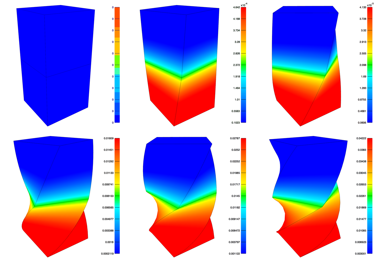
The maximum Green-Lagrange shear strain after twisting the top face by \(\pi\) radians. Note the top layer is 2X stiffer than the bottom layer.
Biphasic Hex20
Most steps are similar to the Elastic Hex20 example. We instead instantiate a pyfebio BiphasicModel, which sets the module to “biphasic”, the analysis to “TRANSIENT”, and the solver type to “biphasic”. We assign a BiphasicMaterial with a NeoHookean solid phase and ConstantIsoPerm as the permeability. The bottom nodes are fixed in space, a BCZeroFluidPressure boundary condition to allow free-draining on the top surface, and a BCPrescribedDisplacement in the z direction for the top nodes.
from meshio.gmsh import read

import pyfebio as feb

# import mesh from gmsh format
from_gmsh = read("../../assets/gmsh/hex20.msh")
# translate meshio mesh to febio mesh
mesh = feb.mesh.translate_meshio(from_gmsh)

# initialize a biphasic febio modelk
my_model = feb.model.BiphasicModel(mesh_=mesh)
assert my_model.control_ is not None
my_model.control_.step_size = 0.1
my_model.control_.time_stepper = feb.control.TimeStepper(dtmax=feb.control.TimeStepValue(text=1.0))

# loop over Elements (parts) and assign biphasic materials
# and also assign solid domains
for i, part in enumerate(my_model.mesh_.elements):
    mat = feb.material.BiphasicMaterial(
        name=part.name,
        solid=feb.material.NeoHookean(),
        permeability=feb.material.ConstantIsoPerm(perm=feb.material.MaterialParameter(text=1e-3 * (i + 1))),
    )
    my_model.material_.add_material(mat)
    my_model.meshdomains_.add_solid_domain(feb.meshdomains.SolidDomain(name=part.name, mat=part.name))

# fix the bottom nodes in space
fix_bottom = my_model.boundary_.add_bc(feb.boundary.BCZeroDisplacement(node_set="bottom", x_dof=1, y_dof=1, z_dof=1))

# set zero fluid pressure bc on bottom nodes to allow for free-draining
drain_bottom = my_model.boundary_.add_bc(feb.boundary.BCZeroFluidPressure(node_set="bottom"))

# set zero fluid pressure bc on top nodes to allow for free-draining
drain_top = my_model.boundary_.add_bc(feb.boundary.BCZeroFluidPressure(node_set="top"))

# displace the top nodes by -0.5 mm in z
move_top = my_model.boundary_.add_bc(
    feb.boundary.BCPrescribedDisplacement(node_set="top", dof="z", value=feb.boundary.Value(lc=1, text=-0.5))
)

# load curve to apply displacement
my_model.loaddata_.add_load_curve(feb.loaddata.LoadCurve(id=1, points=feb.loaddata.CurvePoints(points=["0.0,0.0", "0.1,1.0", "10.0,1.0"])))

# add some additonial variables to plotfile
my_model.output_.add_plotfile(
    feb.output.OutputPlotfile(
        all_vars=[
            feb.output.Var(type="displacement"),
            feb.output.Var(type="effective fluid pressure"),
            feb.output.Var(type="nodal fluid flux"),
            feb.output.Var(type="Lagrange strain"),
        ]
    )
)

# save the model to disk
my_model.save("biphasic_hex20.feb")
# run the model
feb.model.run_model("biphasic_hex20.feb")
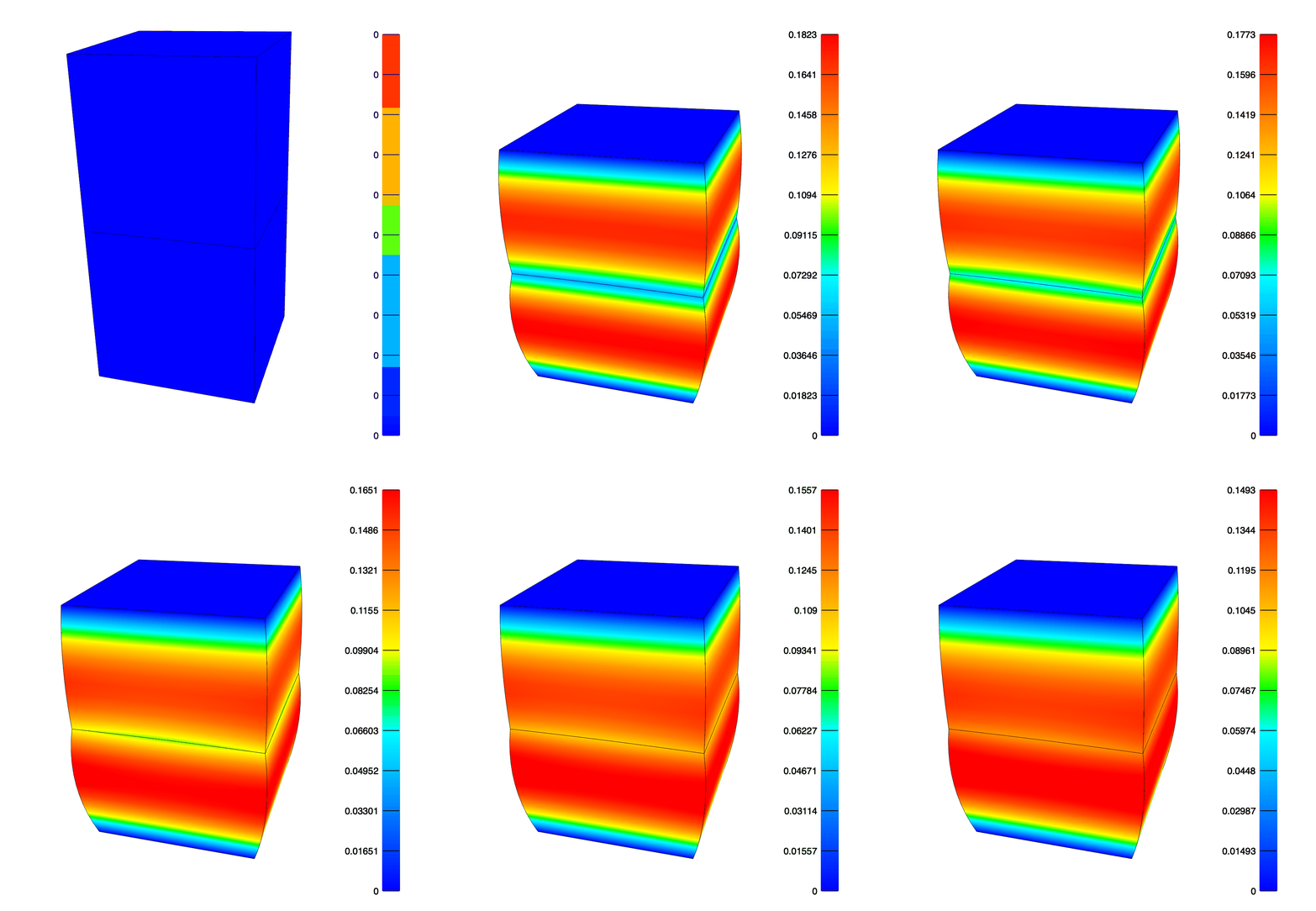
The effective fluid pressure after compressing the top face by 0.5mm in 0.1 seconds and then holding for 9.9 seconds. Note that the top element has twice the permeability of the bottom, hence the asymmetry in fluid pressure and deformation.
Sliding Contact
This example demonstrates sliding contact. This requires the definition of a SurfacePair, which is then referenced in the SlidingElastic contact definition. We enforce the contact constraint with the augmented Lagrange multiplier method by setting laugon=”AUGLAG”. We also set two_pass=1, which helps reduce penetration at the sharp edges of this very coarse mesh.
import meshio

import pyfebio as feb

# read a 27 node hex mesh in gmsh format
from_gmsh = meshio.gmsh.read("../../assets/gmsh/hex27_contact.msh")
# translate gmsh meshio object to an febio mesh
mesh = feb.mesh.translate_meshio(from_gmsh)

# initialize and febio model with default settings
my_model = feb.model.Model(mesh_=mesh)

# loop over the mesh Elements (parts) and assign materials
# and solid domains
for part in my_model.mesh_.elements:
    mat = feb.material.NeoHookean(
        name=part.name,
        E=feb.material.MaterialParameter(text=1.0),
        v=feb.material.MaterialParameter(text=0.3),
    )
    my_model.material_.add_material(mat)
    my_model.meshdomains_.add_solid_domain(feb.meshdomains.SolidDomain(name=part.name, mat=part.name))

# add a surface pair for the contact definition
my_model.mesh_.add_surface_pair(feb.mesh.SurfacePair(name="contact", primary="bottom-box-top", secondary="top-box-bottom"))

# fix the bottom nodes of the bottom box in space
my_model.boundary_.add_bc(feb.boundary.BCZeroDisplacement(node_set="bottom-box-bottom", x_dof=1, y_dof=1, z_dof=1))

# fix the top nodes of the top box in the y dimension
my_model.boundary_.add_bc(feb.boundary.BCZeroDisplacement(node_set="top-box-top", x_dof=0, y_dof=1, z_dof=0))

# move the top nodes of the top box in the the dimension
my_model.boundary_.add_bc(
    feb.boundary.BCPrescribedDisplacement(node_set="top-box-top", dof="z", value=feb.boundary.Value(lc=1, text=-0.15))
)

# move the top nodes of the top box in the x dimension
my_model.boundary_.add_bc(feb.boundary.BCPrescribedDisplacement(node_set="top-box-top", dof="x", value=feb.boundary.Value(lc=1, text=0.3)))
# add a sliding contact definition. enforce it with augmented lagrangian multiplier
my_model.contact_.add_contact(
    feb.contact.SlidingElastic(name="sliding_contact", surface_pair="contact", auto_penalty=1, laugon="AUGLAG", two_pass=1)
)

# load curve controlling the top nodes displacement
my_model.loaddata_.add_load_curve(feb.loaddata.LoadCurve(id=1, points=feb.loaddata.CurvePoints(points=["0,0", "1,1"])))

# add variables to the plotfile output
my_model.output_.add_plotfile(
    feb.output.OutputPlotfile(
        all_vars=[
            feb.output.Var(type="displacement"),
            feb.output.Var(type="contact pressure"),
            feb.output.Var(type="contact gap"),
            feb.output.Var(type="Lagrange strain"),
        ]
    )
)
# save the model to disk
my_model.save("contact.feb")
# run the model
feb.model.run_model("contact.feb")
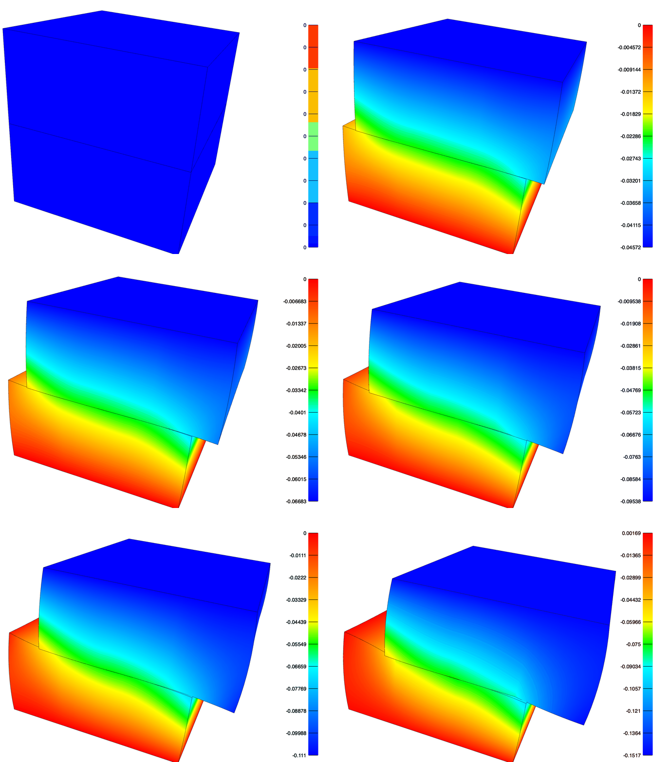
The z-displacement resulting from the contact simulation. Note the nodal penetration near the sharp edge due to the coarse mesh size. This is more severe if the penalty method is used or two_pass is turned off.
Adaptive Remeshing
FEBio has several implementations of adaptive remeshing. This example demonstrates an adaptor that will refine a hex8 mesh to reduce the stress error in the bottom-layer.
import meshio

import pyfebio as feb

# import an 8 node hex mesh in gmsh format
from_gmsh = meshio.gmsh.read("../../assets/gmsh/hex8.msh")

# convert the meshio object to febio mesh
mesh = feb.mesh.translate_meshio(from_gmsh)

# crete a base febio model but override the control section to have constant time step
my_model = feb.model.Model(mesh_=mesh, control_=feb.control.Control(time_steps=10, step_size=0.1, time_stepper=None))

# loop over all Elements in the mesh and assign materials and solid domains
for i, part in enumerate(my_model.mesh_.elements):
    mat = feb.material.NeoHookean(
        name=part.name,
        E=feb.material.MaterialParameter(text=10.0 * (i + 1)),
        v=feb.material.MaterialParameter(text=0.3),
    )
    my_model.material_.add_material(mat)
    my_model.meshdomains_.add_solid_domain(feb.meshdomains.SolidDomain(name=part.name, mat=part.name))

# fix the bottom nodes
fix_bottom = my_model.boundary_.add_bc(feb.boundary.BCZeroDisplacement(node_set="bottom", x_dof=1, y_dof=1, z_dof=1))

# displace the top nodes in z by -0.5 mm
move_top = my_model.boundary_.add_bc(
    feb.boundary.BCPrescribedDisplacement(node_set="top", dof="z", value=feb.boundary.Value(lc=1, text=0.5))
)

# load curve controlling the top nodes displacement
my_model.loaddata_.add_load_curve(feb.loaddata.LoadCurve(id=1, points=feb.loaddata.CurvePoints(points=["0.0,0.0", "1.0,1.0"])))

# creat are mesh adaptor to refine the mesh based
# on the stress error criterion
adaptor = feb.meshadaptor.HexRefineAdaptor(
    elem_set="bottom-layer",
    max_iters=1,
    max_elements=10000,
    criterion=feb.meshadaptor.RelativeErrorCriterion(error=0.01, data=feb.meshadaptor.StressCriterion()),
)
my_model.meshadaptor_.add_adaptor(adaptor)

# we have to add the stress error output to the plotfile so our mesh
# adaptor works
my_model.output_.add_plotfile(
    feb.output.OutputPlotfile(
        all_vars=[
            feb.output.Var(type="displacement"),
            feb.output.Var(type="stress error"),
        ]
    )
)

# save our madel to disk
my_model.save("mesh_adapt.feb")
# run the model
feb.model.run_model("mesh_adapt.feb")
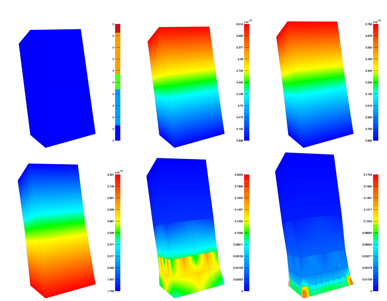
The hex mesh adaptively refines to reduce the stress error in the bottom-layer. Note the greatest refinement occurs at the necking corners.
Three Cylinder Joint
This example demonstrates the use of rigid connectors to create a three cylinder linkage, which is a popular approach to modeling joint dynamics.
import pyfebio as feb

# manually create the nodes
all_nodes = [
    feb.mesh.Node(id=1, text="-2.0,-1.0,-10"),
    feb.mesh.Node(id=2, text="2.0,-1.0,-10"),
    feb.mesh.Node(id=3, text="2.0,1.0,-10"),
    feb.mesh.Node(id=4, text="-2.0,1.0,-10"),
    feb.mesh.Node(id=5, text="-2.0,-1.0,0"),
    feb.mesh.Node(id=6, text="2.0,-1.0,0"),
    feb.mesh.Node(id=7, text="2.0,1.0,0"),
    feb.mesh.Node(id=8, text="-2.0,1.0,0"),
    feb.mesh.Node(id=9, text="-2.0,-1.0,0"),
    feb.mesh.Node(id=10, text="2.0,-1.0,0"),
    feb.mesh.Node(id=11, text="2.0,1.0,0"),
    feb.mesh.Node(id=12, text="-2.0,1.0,0"),
    feb.mesh.Node(id=13, text="-2.0,-1.0,10"),
    feb.mesh.Node(id=14, text="2.0,-1.0,10"),
    feb.mesh.Node(id=15, text="2.0,1.0,10"),
    feb.mesh.Node(id=16, text="-2.0,1.0,10"),
]

# create a Nodes object
nodes = feb.mesh.Nodes(name="Nodes", all_nodes=all_nodes)

# create Hex8Element for rigid bodies
# each of these is a separate Elements object
# so they are unique parts
body_a = feb.mesh.Elements(name="BodyA", type="hex8", all_elements=[feb.mesh.Hex8Element(id=1, text="1,2,3,4,5,6,7,8")])
body_b = feb.mesh.Elements(name="BodyB", type="hex8", all_elements=[feb.mesh.Hex8Element(id=2, text="9,10,11,12,13,14,15,16")])

# create the base model
my_model = feb.model.Model()
# add the Nodes
my_model.mesh_.add_node_domain(nodes)
# add the Elements (parts)
my_model.mesh_.add_element_domain(body_a)
my_model.mesh_.add_element_domain(body_b)

# create rigid body materials for BodyA and BodyB
my_model.material_.add_material(feb.material.RigidBody(name="BodyA", center_of_mass="0,0,0"))
my_model.material_.add_material(feb.material.RigidBody(name="BodyB", center_of_mass="0,0,0"))
# assign solid domains to the rigid bodies
my_model.meshdomains_.add_solid_domain(feb.meshdomains.SolidDomain(name="BodyA", mat="BodyA"))
my_model.meshdomains_.add_solid_domain(feb.meshdomains.SolidDomain(name="BodyB", mat="BodyB"))

# we need two more rigid bodies for the purpose of creating our
# three cylinder linkage. We use the convenience function
# add_simple_rigid_body() to create these
my_model.add_simple_rigid_body(origin=(0.0, 0.0, 0.0), name="GhostA")
my_model.add_simple_rigid_body(origin=(0.0, 0.0, 0.0), name="GhostB")

# fix BodyA in space
my_model.rigid_.add_rigid_bc(feb.rigid.RigidFixed(rb="BodyA", Rx_dof=1, Ry_dof=1, Rz_dof=1, Ru_dof=1, Rw_dof=1, Rv_dof=1))

# define a RigidCylindricalJoint connector between BodyA and GhostA
# this is the internal-external rotation / inferior-superior translation axis
# prescribe rotation and translation
my_model.rigid_.add_rigid_connector(
    feb.rigid.RigidCylindricalJoint(
        name="IERot_ISTranslation",
        body_a="BodyA",
        body_b="GhostA",
        joint_axis="0.0,0.0,1.0",
        transverse_axis="1.0,0.0,0.0",
        prescribed_rotation=1,
        prescribed_translation=1,
        rotation=feb.rigid.Value(lc=1, text=1.57),
        translation=feb.rigid.Value(lc=2, text=1.0),
    )
)
# define a RigidCylindricalJoint connector between GhostA and GhostB
# this is the varus-valgus rotation / anterior-posterior translation axis
# prescribe rotation and translation
my_model.rigid_.add_rigid_connector(
    feb.rigid.RigidCylindricalJoint(
        name="VVRot_APTranslation",
        body_a="GhostA",
        body_b="GhostB",
        joint_axis="0.0,1.0,0.0",
        transverse_axis="1.0,0.0,0.0",
        prescribed_rotation=1,
        prescribed_translation=1,
        rotation=feb.rigid.Value(lc=3, text=1.57),
        translation=feb.rigid.Value(lc=4, text=1.0),
    )
)
# define a RigidCylindricalJoint connector between GhostB and BodyB
# this is the flexion-extension rotation / medial-lateral translation axis
# prescribe rotation and translation
my_model.rigid_.add_rigid_connector(
    feb.rigid.RigidCylindricalJoint(
        name="Flexion_MLTranslation",
        body_a="GhostB",
        body_b="BodyB",
        joint_axis="1.0,0.0,0.0",
        transverse_axis="0.0,0.0,1.0",
        prescribed_rotation=1,
        prescribed_translation=1,
        rotation=feb.rigid.Value(lc=5, text=1.57),
        translation=feb.rigid.Value(lc=6, text=1.0),
    )
)

# load curve for internal-external rotation
my_model.loaddata_.add_load_curve(
    feb.loaddata.LoadCurve(id=1, points=feb.loaddata.CurvePoints(points=["0.0,0.0", "0.5,1.0", "1.5,-1.0", "2.0,0.0"]))
)
# load curve for inferior-superior translation
my_model.loaddata_.add_load_curve(
    feb.loaddata.LoadCurve(id=2, points=feb.loaddata.CurvePoints(points=["0.0,0.0", "2.0,0.0", "2.5,1.0", "3.5,-1.0", "4.0,0.0"]))
)
# load curve for varus-valgus rotation
my_model.loaddata_.add_load_curve(
    feb.loaddata.LoadCurve(id=3, points=feb.loaddata.CurvePoints(points=["0.0,0.0", "4.0,0.0", "4.5,1.0", "5.5,-1.0", "6.0,0.0"]))
)
# load curve for anterior-posterior translation
my_model.loaddata_.add_load_curve(
    feb.loaddata.LoadCurve(id=4, points=feb.loaddata.CurvePoints(points=["0.0,0.0", "6.0,0.0", "6.5,1.0", "7.5,-1.0", "8.0,0.0"]))
)
# load curve for flexion-extension rotation
my_model.loaddata_.add_load_curve(
    feb.loaddata.LoadCurve(id=5, points=feb.loaddata.CurvePoints(points=["0.0,0.0", "8.0,0.0", "8.5,1.0", "9.5,-1.0", "10.0,0.0"]))
)
# load curve for medial-lateral translation
my_model.loaddata_.add_load_curve(
    feb.loaddata.LoadCurve(id=6, points=feb.loaddata.CurvePoints(points=["0.0,0.0", "10.0,0.0", "10.5,1.0", "11.5,-1.0", "12.0,0.0"]))
)

# must point load curve; note interpolate="STEP"
my_model.loaddata_.add_load_curve(
    feb.loaddata.LoadCurve(
        id=7,
        interpolate="STEP",
        points=feb.loaddata.CurvePoints(points=[f"{i * 0.25},0.25" for i in range(48)]),
    )
)


# change the number of time steps and step_size
# to cover 12 second simulation time
my_model.control_ = feb.control.Control(time_steps=24, step_size=0.5)

# set dtmax of time_stepper to must point load curve
# this guarantees we have a solution at the beginning and end of
# each dof trajectory
my_model.control_.time_stepper.dtmax = feb.control.TimeStepValue(lc=7, text=0.5)

# save and run the model
my_model.save("three_cylinder_joint.feb")
feb.model.run_model("three_cylinder_joint.feb")
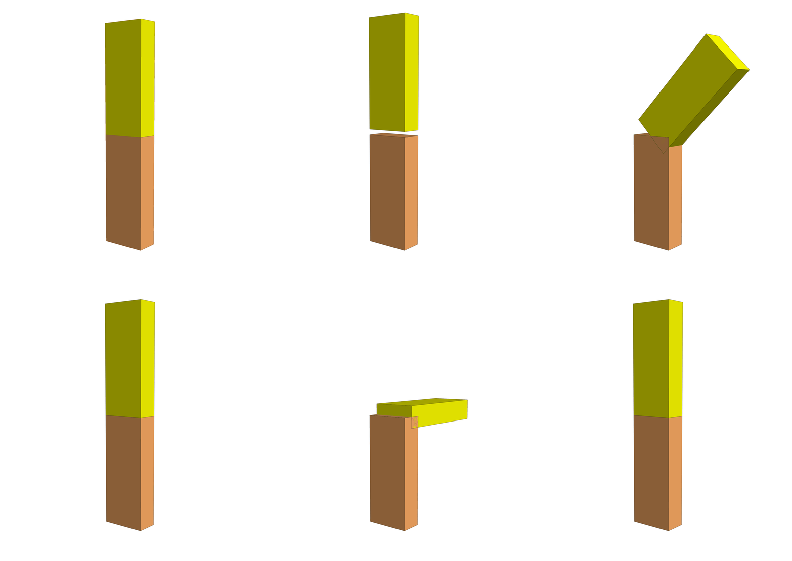
Enforcing \(\pm \frac{\pi}{2}\) radian rotations about the flexion-extension, varus-valgus, and internal-external rotation axes, and \(\pm 1.0\) inferior-superior, medial-lateral, and anterior-posterior translations with rigid connectors. The GhostA and GhostB rigid bodies are hidden.
XPLT Conversion to HDF5
This example demonstrates the conversion of XPLT files to HDF5 format.
In a script:
from pyfebio import xplt

xplt.to_hdf5(inputfile="../../assets/elastic_hex20.xplt", outputfile="elastic_hex20.hdf5")
From the command line in src/examples directory:
python -m pyfebio.xplt ../../assets/elastic_hex20.xplt elastic_hex20.hdf5
One can then interact with the HDF5 file using the h5py package.
For example,
import h5py


def print_datasets(name, obj):
    if isinstance(obj, h5py.Dataset):
        print(name, f"shape: {obj.shape}", f"dtype: {obj.dtype}")


f = h5py.File("elastic_hex20.hdf5", "r")
# view all the datasets and their shape and dtype
f.visititems(print_datasets)

# shared attributes are stored at the appropriate parent group
# e.g. the time at a given state can be accessed as follows:
print("\n Time at state 5")
print(f["/states/5"].attrs["time"])

# to view the data in a Dataset
print("\n Displacement at state 5")
print(f["/states/5/node_data/displacement/1"][:])  # type: ignore

# this is simply a numpy array so we can also slice it
print("\n Displacement at state 5 of first 2 nodes")
print(f["/states/5/node_data/displacement/1"][0:2, :])  # type: ignore
# the nice thing about this though is HDF5 uses lazy loading
# which means that the data is not loaded into memory until it is accessed
# this is useful for large datasets that do not fit into memory

f.close()
Output:
meshes/0/domains/bottom-layer shape: (1, 21) dtype: int32
meshes/0/domains/top-layer shape: (1, 21) dtype: int32
meshes/0/elementsets/bottom-layer shape: (1,) dtype: int32
meshes/0/elementsets/top-layer shape: (1,) dtype: int32
meshes/0/nodes shape: (32,) dtype: [('id', '<i4'), ('x', '<f4'), ('y', '<f4'), ('z', '<f4')]
meshes/0/nodesets/1 shape: (32,) dtype: int32
meshes/0/nodesets/back shape: (13,) dtype: int32
meshes/0/nodesets/bottom shape: (8,) dtype: int32
meshes/0/nodesets/front shape: (13,) dtype: int32
meshes/0/nodesets/left shape: (13,) dtype: int32
meshes/0/nodesets/right shape: (13,) dtype: int32
meshes/0/nodesets/top shape: (8,) dtype: int32
meshes/0/surfaces/back shape: (2, 10) dtype: int32
meshes/0/surfaces/bottom shape: (1, 10) dtype: int32
meshes/0/surfaces/front shape: (2, 10) dtype: int32
meshes/0/surfaces/left shape: (2, 10) dtype: int32
meshes/0/surfaces/right shape: (2, 10) dtype: int32
meshes/0/surfaces/top shape: (1, 10) dtype: int32
states/0/element_data/stress/bottom-layer shape: (1, 6) dtype: float32
states/0/element_data/stress/top-layer shape: (1, 6) dtype: float32
states/0/mesh/element_state shape: (2,) dtype: int32
states/0/node_data/displacement/1 shape: (32, 3) dtype: float32
states/1/element_data/stress/bottom-layer shape: (1, 6) dtype: float32
states/1/element_data/stress/top-layer shape: (1, 6) dtype: float32
states/1/mesh/element_state shape: (2,) dtype: int32
states/1/node_data/displacement/1 shape: (32, 3) dtype: float32
states/2/element_data/stress/bottom-layer shape: (1, 6) dtype: float32
states/2/element_data/stress/top-layer shape: (1, 6) dtype: float32
states/2/mesh/element_state shape: (2,) dtype: int32
states/2/node_data/displacement/1 shape: (32, 3) dtype: float32
states/3/element_data/stress/bottom-layer shape: (1, 6) dtype: float32
states/3/element_data/stress/top-layer shape: (1, 6) dtype: float32
states/3/mesh/element_state shape: (2,) dtype: int32
states/3/node_data/displacement/1 shape: (32, 3) dtype: float32
states/4/element_data/stress/bottom-layer shape: (1, 6) dtype: float32
states/4/element_data/stress/top-layer shape: (1, 6) dtype: float32
states/4/mesh/element_state shape: (2,) dtype: int32
states/4/node_data/displacement/1 shape: (32, 3) dtype: float32
states/5/element_data/stress/bottom-layer shape: (1, 6) dtype: float32
states/5/element_data/stress/top-layer shape: (1, 6) dtype: float32
states/5/mesh/element_state shape: (2,) dtype: int32
states/5/node_data/displacement/1 shape: (32, 3) dtype: float32

Time at state 5
[1.]

Displacement at state 5
[[ 0.0000000e+00  0.0000000e+00  0.0000000e+00]
[ 1.1734079e+00  3.4618369e-01  4.2698154e-04]
[ 3.4618369e-01 -1.1734079e+00  4.2698154e-04]
[ 0.0000000e+00  0.0000000e+00  0.0000000e+00]
[ 0.0000000e+00  0.0000000e+00  0.0000000e+00]
[-3.4618369e-01  1.1734079e+00  4.2698154e-04]
[-1.1734079e+00 -3.4618369e-01  4.2698154e-04]
[ 0.0000000e+00  0.0000000e+00  0.0000000e+00]
[ 1.0007957e+00  9.9920303e-01  0.0000000e+00]
[ 9.9920303e-01 -1.0007957e+00  0.0000000e+00]
[-9.9920303e-01  1.0007957e+00  0.0000000e+00]
[-1.0007957e+00 -9.9920303e-01  0.0000000e+00]
[ 6.8272942e-01 -1.3276277e-01 -1.4378540e-03]
[ 7.6155305e-01 -4.1322845e-01  8.6941756e-03]
[-1.3276277e-01 -6.8272942e-01 -1.4378540e-03]
[ 0.0000000e+00  0.0000000e+00  0.0000000e+00]
[ 1.3276277e-01  6.8272942e-01 -1.4378540e-03]
[-7.6155305e-01  4.1322845e-01  8.6941756e-03]
[-6.8272942e-01  1.3276277e-01 -1.4378540e-03]
[ 0.0000000e+00  0.0000000e+00  0.0000000e+00]
[ 0.0000000e+00  0.0000000e+00  0.0000000e+00]
[ 4.1322845e-01  7.6155305e-01  8.6941756e-03]
[ 0.0000000e+00  0.0000000e+00  0.0000000e+00]
[-4.1322845e-01 -7.6155305e-01  8.6941756e-03]
[ 1.1713763e+00  6.9261616e-01  2.4284013e-03]
[ 9.9999934e-01 -7.9632644e-04  0.0000000e+00]
[ 6.9261616e-01 -1.1713763e+00  2.4284013e-03]
[-6.9261616e-01  1.1713763e+00  2.4284013e-03]
[-9.9999934e-01  7.9632644e-04  0.0000000e+00]
[-1.1713763e+00 -6.9261616e-01  2.4284013e-03]
[ 7.9632644e-04  9.9999934e-01  0.0000000e+00]
[-7.9632644e-04 -9.9999934e-01  0.0000000e+00]]

Displacement at state 5 of first 2 nodes
[[0.0000000e+00 0.0000000e+00 0.0000000e+00]
[1.1734079e+00 3.4618369e-01 4.2698154e-04]]